Cross-mapping biodiversity metrics across spaces
Bruno Vilela
2025-07-07
Source:vignettes/Cross-mapping-biodiversity-metrics-Phyllomedusa.Rmd
Cross-mapping-biodiversity-metrics-Phyllomedusa.RmdOverview
This vignette demonstrates cross-mapping of
biodiversity metrics between environmental,
geographic, and attribute (trait)
spaces using letsR. We:
- Build an environmental-space PAM from Phyllomedusa data;
- Compute per-cell descriptors in environmental space;
- Summarize those descriptors to species level; and
- Project (cross-map) a chosen environmental metric into geographic and attribute spaces via the package connectors.
Data and environmental PAM (example with Phyllomedusa)
First we create a geographic and environmental PAM as described in previous articles.
library(letsR)

# Occurrences and climate
data("Phyllomedusa"); data("prec"); data("temp")
prec <- terra::unwrap(prec); temp <- terra::unwrap(temp)

# Geographic PAM (keep empty cells)
PAM  <- lets.presab(Phyllomedusa, remove.cells = FALSE)

# Keep terrestrial landmasses for plotting and binning consistency
wrld_simpl <- get(utils::data("wrld_simpl", package = "letsR"))
PAM <- lets.pamcrop(PAM, terra::vect(wrld_simpl))

# Environmental variables matrix (per geographic cell)
envs <- lets.addvar(PAM, c(temp, prec), onlyvar = TRUE)
colnames(envs) <- c("Temperature", "Precipitation")

# Environmental-space PAM (envPAM)
env_obj <- lets.envpam(PAM, envs, n_bins = 30, remove.cells = FALSE)

# Plot
lets.plot.envpam(env_obj, world = TRUE)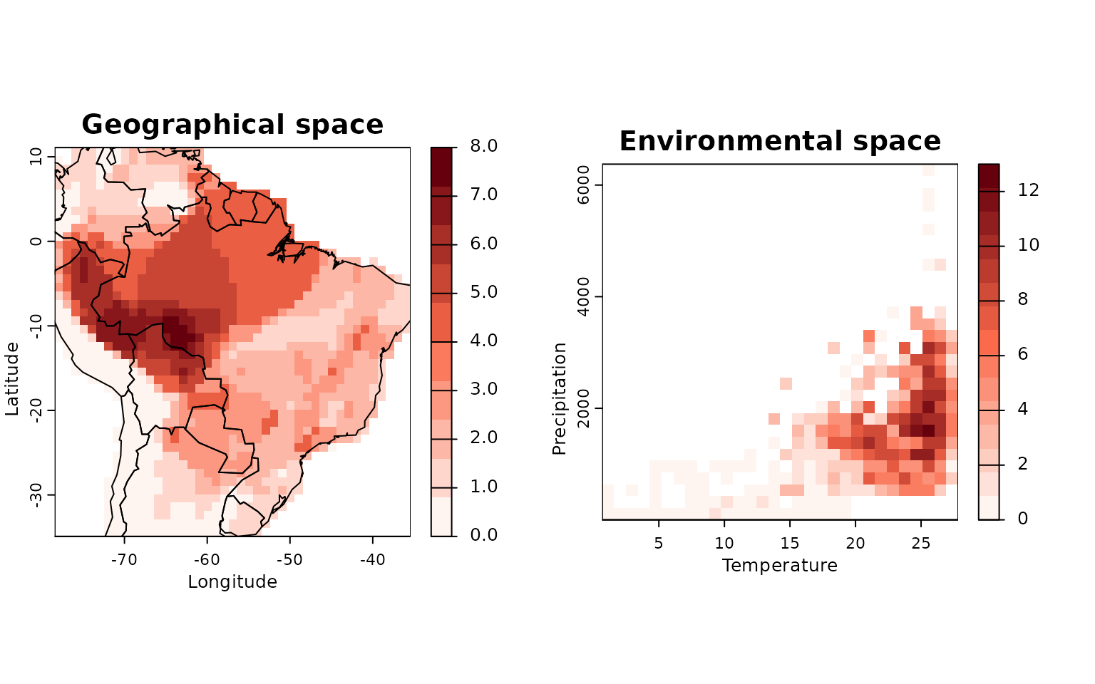
Environmental descriptors per environmental cell
# Compute env-space descriptors (centrality, border, isolation, etc.)
env_cells <- lets.envcells(env_obj, perc = 0.2)

head(env_cells)
#>   Cell_env Frequency Area Isolation (Min.) Isolation (1st Qu.)
#> 1        1         0   NA               NA                  NA
#> 2        2         0   NA               NA                  NA
#> 3        3         0   NA               NA                  NA
#> 4        4         0   NA               NA                  NA
#> 5        5         0   NA               NA                  NA
#> 6        6         0   NA               NA                  NA
#>   Isolation (Median) Isolation (Mean) Isolation (3rd Qu.) Isolation (Max.)
#> 1                 NA               NA                  NA               NA
#> 2                 NA               NA                  NA               NA
#> 3                 NA               NA                  NA               NA
#> 4                 NA               NA                  NA               NA
#> 5                 NA               NA                  NA               NA
#> 6                 NA               NA                  NA               NA
#>   Weighted Mean Distance to midpoint Mean Distance to midpoint
#> 1                          -3.730908                 -3.457246
#> 2                          -3.646836                 -3.382386
#> 3                          -3.564523                 -3.309862
#> 4                          -3.484092                 -3.239832
#> 5                          -3.405677                 -3.172460
#> 6                          -3.329421                 -3.107918
#>   Minimum Zero Distance Minimum 20% Zero Distance Distance to MCP border
#> 1                     0                 0.9362266                      0
#> 2                     0                 0.8700119                      0
#> 3                     0                 0.8136812                      0
#> 4                     0                 0.7676179                      0
#> 5                     0                 0.7323872                      0
#> 6                     0                 0.7068043                      0
#>   Frequency Weighted Distance
#> 1                    3.800462
#> 2                    3.718461
#> 3                    3.638213
#> 4                    3.559825
#> 5                    3.483411
#> 6                    3.409092
Summarize those per-cell descriptors to species level by aggregating across the environmental cells each species occupies:
# Species-level summaries (e.g., mean across occupied env cells)
env_by_species <- lets.summaryze.cells(env_obj, env_cells, func = mean)

head(env_by_species)
#>                    Species Frequency         Area Isolation (Min.)
#> 1    Phyllomedusa araguari   9.00000  99942160705         97052.27
#> 2 Phyllomedusa atelopoides  25.38889 310216725731        109736.78
#> 3      Phyllomedusa ayeaye  11.50000 129979311887         99631.44
#> 4      Phyllomedusa azurea  11.59091 137178852573        130717.35
#> 5     Phyllomedusa bahiana  11.91667 142112800724        136522.70
#> 6      Phyllomedusa baltea  19.00000 233017982880        110574.31
#>   Isolation (1st Qu.) Isolation (Median) Isolation (Mean) Isolation (3rd Qu.)
#> 1            494018.8           767952.4         747035.8            923841.2
#> 2            593524.1          1109618.7        1175110.9           1714363.8
#> 3            384047.4           599271.8         667315.7            851729.1
#> 4            462970.6          1391519.0        1328709.9           2016286.4
#> 5            463613.5          1492534.7        1354451.4           2121714.6
#> 6            611182.1          1019632.7        1201164.4           1896221.5
#>   Isolation (Max.) Weighted Mean Distance to midpoint Mean Distance to midpoint
#> 1          1500329                         -0.3188860                -0.1627780
#> 2          3008424                         -0.6007348                -1.0114155
#> 3          1725300                         -0.3310414                -0.1608610
#> 4          3035828                         -0.4455612                -0.7009224
#> 5          2999208                         -0.4520640                -0.6818815
#> 6          2950964                         -0.6779813                -1.0585809
#>   Minimum Zero Distance Minimum 20% Zero Distance Distance to MCP border
#> 1             0.2581989                 0.9296124              0.2581989
#> 2             0.3258642                 1.0476293              0.3258642
#> 3             0.3116736                 0.9521703              0.3116736
#> 4             0.3197515                 1.2125076              0.3197515
#> 5             0.2641105                 1.2398626              0.2641105
#> 6             0.2581989                 0.9893314              0.2581989
#>   Frequency Weighted Distance
#> 1                   0.7555036
#> 2                   0.7967939
#> 3                   0.7590072
#> 4                   0.7875067
#> 5                   0.7752855
#> 6                   0.8278369
We will use one metric from env_by_species(for example,
“Weighted Mean Distance to midpoint”) for cross-mapping.
Attribute-space PAM for Phyllomedusa species
We create a trait grid (attribute space) by simulating two quantitative traits for the species present in our PAM. (Replace with real traits if available.)
set.seed(123)
sp_vec   <- env_by_species$Species                    # species present in PAM
n_sp     <- length(sp_vec)
trait_a  <- rnorm(n_sp)
trait_b  <- trait_a * 0.2 + rnorm(n_sp)               # correlated trait

attr_df  <- data.frame(Species = sp_vec,
                       trait_a  = trait_a,
                       trait_b  = trait_b)

# Attribute-space PAM (AttrPAM)
attr_obj <- lets.attrpam(attr_df, n_bins = 5)

# Richness map in attribute space
lets.plot.attrpam(attr_obj)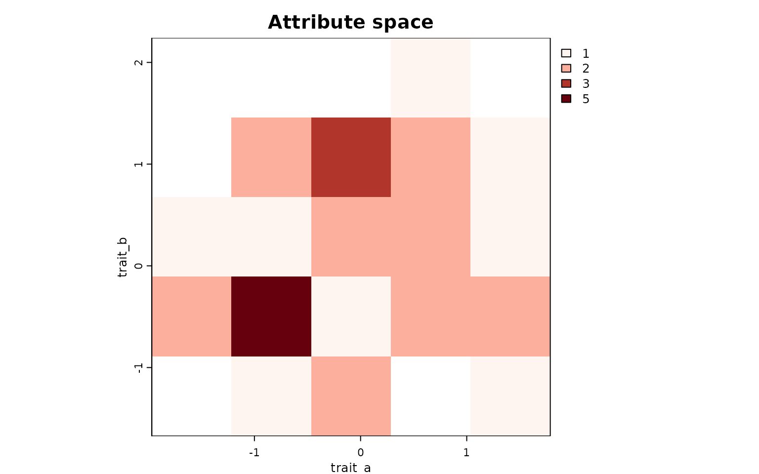
Cross-mapping an environmental metric into geographic and attribute spaces
A. Into geographic space
Project environmental metric to geography:
# Align env-cell descriptors to the order of geographic rows
env_cells_geo <- env_cells[ env_obj$Presence_and_Absence_Matrix_geo[, 1], ]

# Template = geographic richness raster
map_richatt2 <- env_obj$Geo_Richness_Raster
terra::values(map_richatt2) <- NA

# Fill geographic cells with the env-space metric (species-level NOT needed here)
terra::values(map_richatt2)[ env_obj$Presence_and_Absence_Matrix_geo[, 2] ] <-
  env_cells_geo$`Weighted Mean Distance to midpoint`

# Palette and plot
colfunc <- grDevices::colorRampPalette(c("#fff5f0", "#fb6a4a", "#67000d"))
plot(map_richatt2, col = colfunc(200), box = FALSE, axes = FALSE,
     main = "Env centrality (env-space) mapped to geography")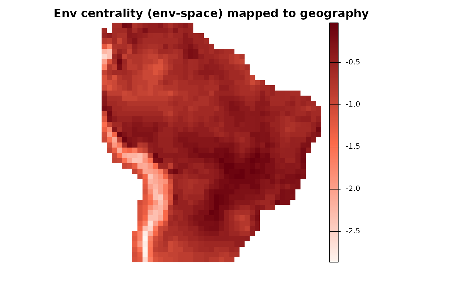
B. Into attribute space
Map the same environmental metric (species-level) into the attribute grid:
met_env <- env_by_species$`Weighted Mean Distance to midpoint`
sp_names <- env_by_species$Species

attr_map <- lets.maplizer.attr(attr_obj, y = met_env, z = sp_names, func = mean)

# Visualize
lets.plot.attrpam(attr_map, mar = c(4,4,4,4))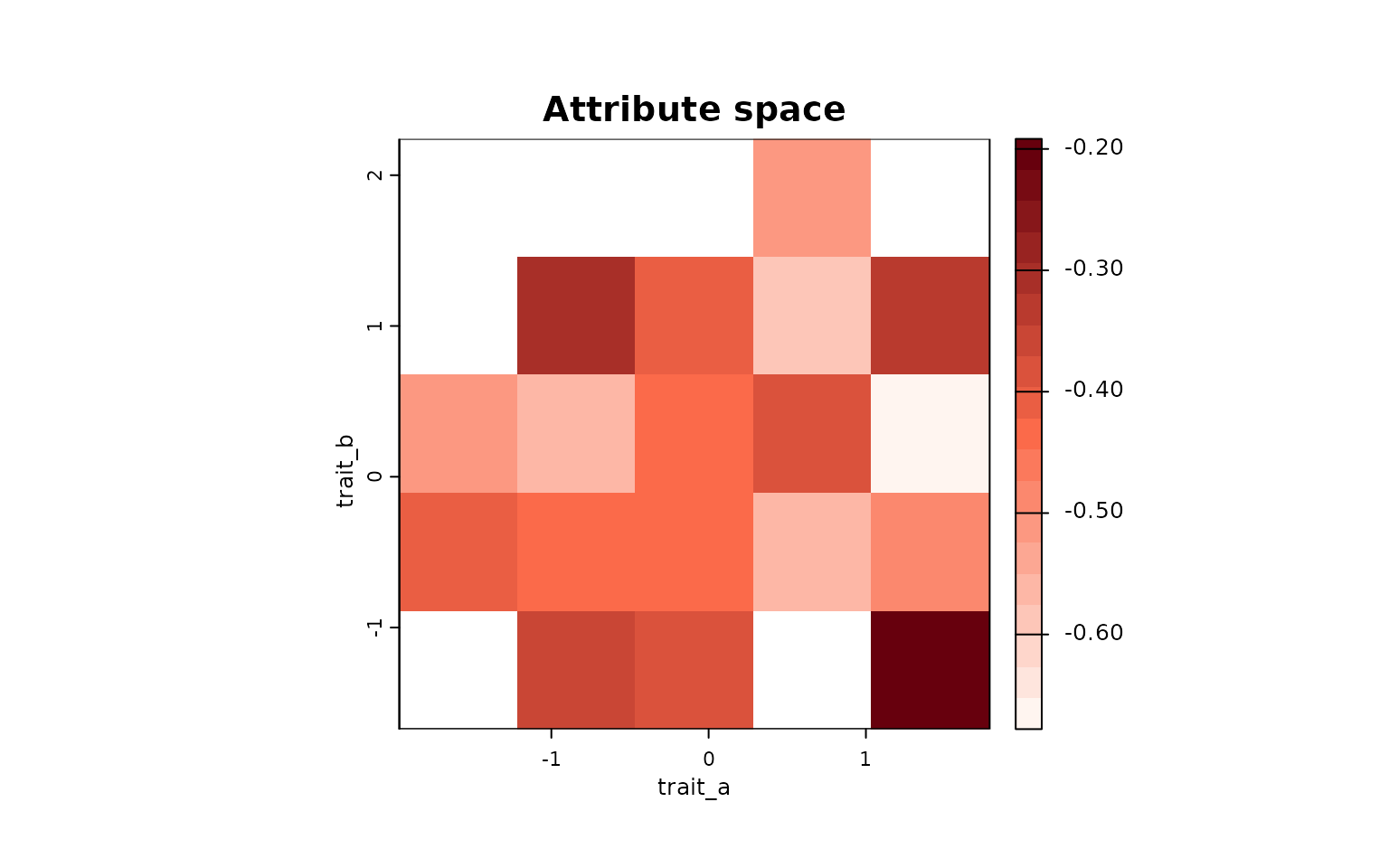
These projections reveal how a descriptor computed in environmental space (centrality) distributes across geographic communities and trait space.
Cross-mapping attribute metrics back to geography
You can compute attribute-space descriptors with
lets.attrcells(attr_obj, ...), summarize them to species
with lets.summarizer.cells(attr_obj, ...), and then project
those species-level metrics to geographic or environmental spaces using
lets.maplizer(...) or
lets.maplizer.env(...).
# Attribute-space descriptors per cell
attr_cells <- lets.attrcells(attr_obj, perc = 0.2)
# Species-level summaries of attribute-space descriptors
attr_by_species <- lets.summaryze.cells(attr_obj, attr_cells, func = mean)
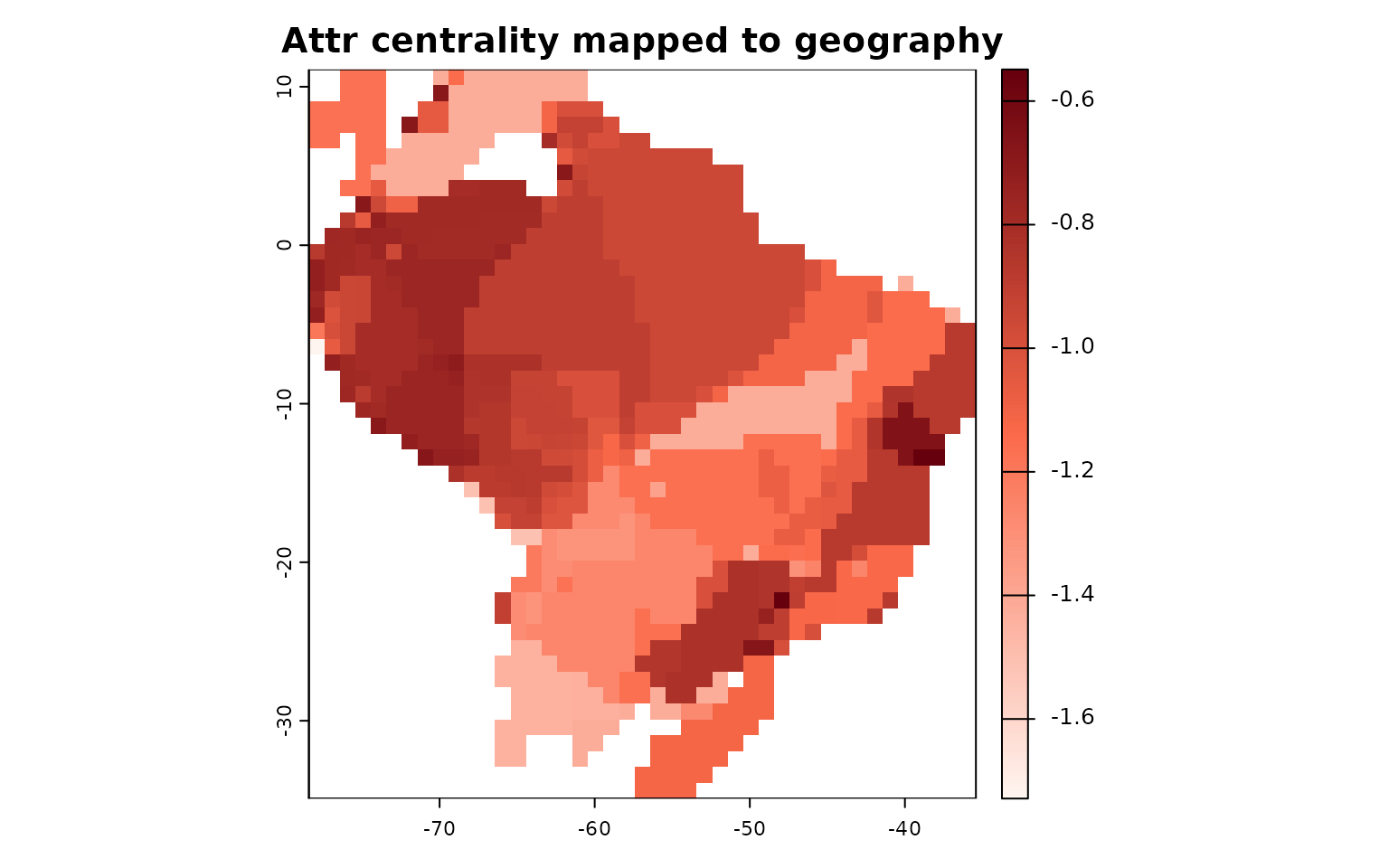
# Example: map an attribute-space centrality back to geography
met_attr <- attr_by_species$`Weighted Mean Distance to midpoint`
geo_from_attr <- lets.maplizer(PAM, y = met_attr, z = attr_by_species$Species, ras = TRUE)
plot(geo_from_attr$Raster, main = "Attr centrality mapped to geography", col = colfunc(200))