Mapping species richness in environmental space
Bruno Vilela
2025-07-07
Source:vignettes/Mapping-species-richness-in-environmental-space.Rmd
Mapping-species-richness-in-environmental-space.RmdSpecies richness and distributions are often analyzed in geographic space. However, understanding biodiversity in environmental space (e.g., across gradients of temperature and precipitation) is fundamental to further understand ecological communities and species distribution.
The new function lets.envpam() from the
letsR package allows users to transform a geographic
presence–absence matrix (PAM) into an environmental-space PAM, by
binning species occurrences according to environmental variables.
Loading data
To start this test we can load our example datasets of
Phyllomedusa frog species occurrences and two environmental
layers: temperature and precipitation.
Note: I recommend to use the latest version of the
letsR package on GitHub
# Load the package
library(letsR)

# Load species occurrences
data("Phyllomedusa")

# Load and unwrap environmental rasters
data("prec")
data("temp")
prec <- unwrap(prec)
temp <- unwrap(temp)
Notice that we need to generate a PAM without removing the cells without records. We can also remove data beyond the geographic limits of continents as the example species are continental organisms.
# Generate a geographic PAM
pam <- lets.presab(Phyllomedusa, remove.cells = FALSE)

# Crop the PAM to the world's landmasses
data("wrld_simpl", package = "letsR")
pam <- lets.pamcrop(pam, terra::vect(wrld_simpl))
Next, we need to add our environmental data to the pam using the
lets.addvar function. Note that we only need to keep the
variables, so set the onlyvar argument
TRUE.
# Extract environmental values
envs <- lets.addvar(pam, c(temp, prec), onlyvar = TRUE)
colnames(envs) <- c("Temperature", "Precipitation")
Creating a PAM in environmental space
We can now combine the PresenceAbsence object and the
envs object to create the presence absence matrix in the
environmental space using the lets.envpamfunction.
# Transform PAM into environmental space
res <- lets.envpam(pam, envs)
The resulting object res contains:
-
Presence_and_Absence_Matrix_env: a matrix of species presence across environmental cells.
-
Presence_and_Absence_Matrix_geo: the original PAM coordinates associated with environmental cells.
-
Env_Richness_Raster: raster showing richness in binned environmental space.
-
Geo_Richness_Raster: the original richness raster in geographic space.
You will note that the environmental and geographic presence–absence
matrices share a common identifier: the Cell_env column.
This linkage allows users to perform integrated analyses, facilitating
the transfer of information between environmental and geographic spaces
in both directions.
res$Presence_and_Absence_Matrix_env[1:5, 1:5]
#>     Cell_env Temperature Precipitation Phyllomedusa araguari
#> 269      269    26.46848      4568.828                     0
#> 387      387    24.65896      3719.128                     0
#> 389      389    26.46848      3719.128                     0
#> 417      417    24.65896      3506.702                     0
#> 418      418    25.56372      3506.702                     0
#>     Phyllomedusa atelopoides
#> 269                        0
#> 387                        0
#> 389                        0
#> 417                        0
#> 418                        0
res$Presence_and_Absence_Matrix_geo[1:5, 1:5]
#>      Cell_env Cell_geo Longitude(x) Latitude(y) Phyllomedusa araguari
#> [1,]      750        3    -75.92399     10.5907                     0
#> [2,]      750        4    -74.92399     10.5907                     0
#> [3,]      715        5    -73.92399     10.5907                     0
#> [4,]      716        6    -72.92399     10.5907                     0
#> [5,]      780        7    -71.92399     10.5907                     0
Visualizing environmental richness
The letsR package also offers a function to plot
richness plot in both environmental and geographic space.
lets.plot.envpam(res,
            world = TRUE)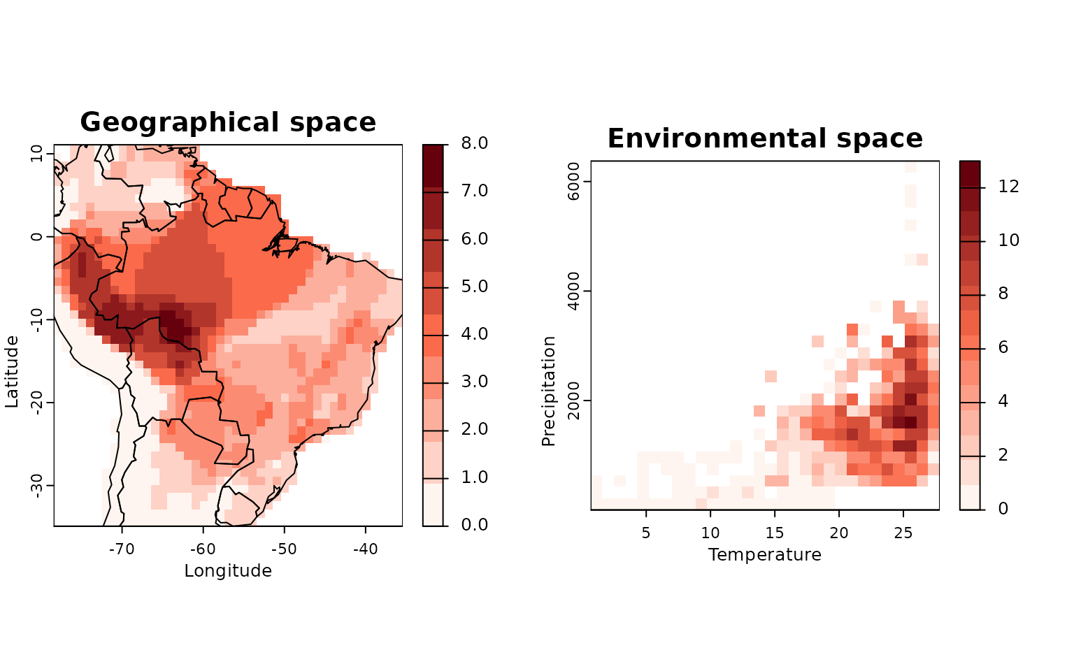
This plot shows species richness both in geographic (left) and environmental (right) space.
Highlighting a single species
To visualize where a specific species occurs in both spaces:
lets.plot.envpam(res, species = "Phyllomedusa atelopoides")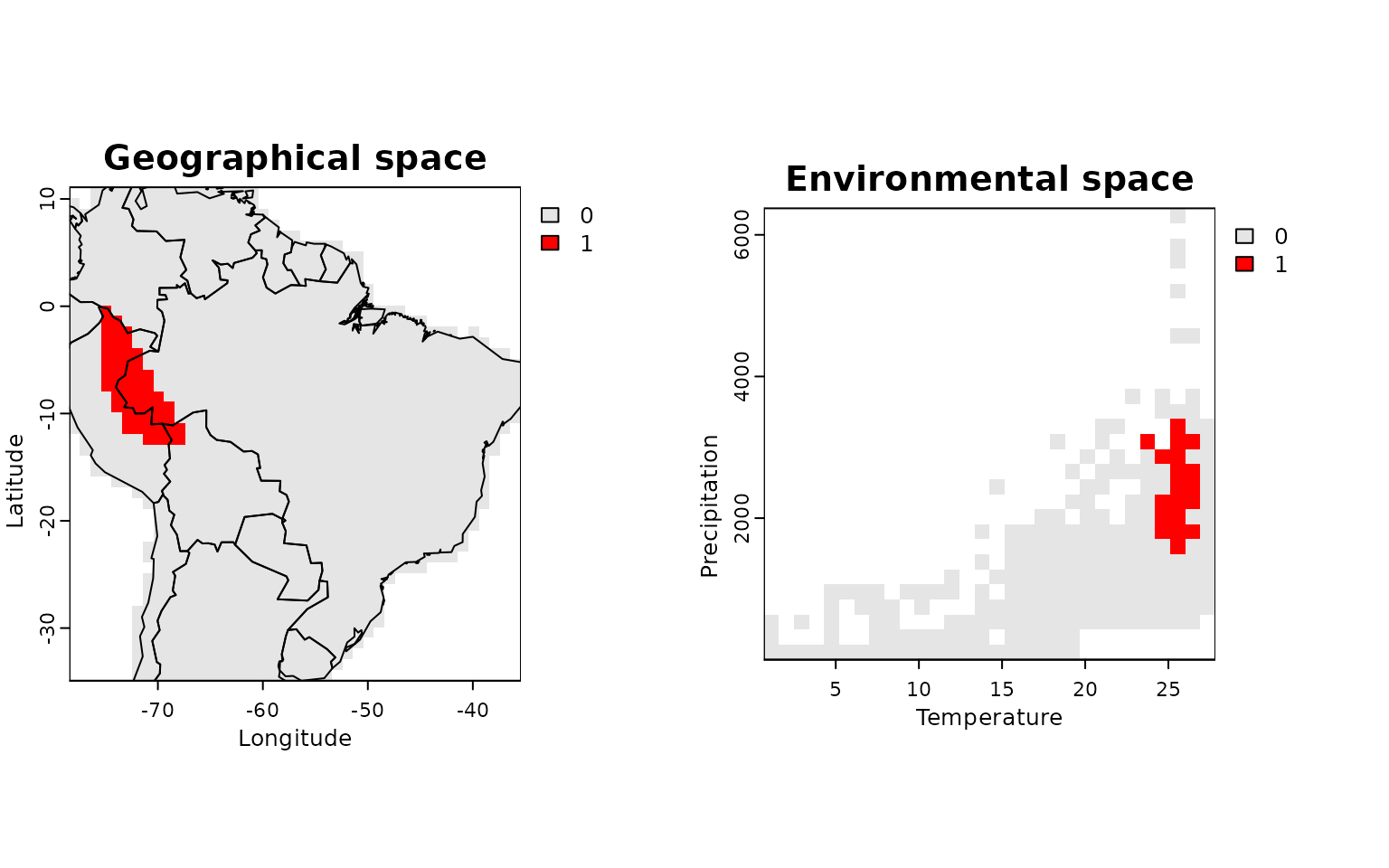
Mapping traits in environmental space
The function lets.maplizer.env also allow users to map
species attributes in both environmental and geographic spaces. Let’s
use the species description date available in the IUCN
example object.
data("IUCN")
# Map mean description year
res_map <- lets.maplizer.env(res,
                             y = IUCN$Description_Year,
                             z = IUCN$Species)
The results are pretty similar to the lets.envpam
results, except that now instead of presence-absence for each species
there will be the summarized attribute. In this case the mean
description year per cell. You can also use the
lets.plot.envpam function to visualize the results (notice
that you cannot plot individual species or cells in this case).
# Plotting trait maps
lets.plot.envpam(res_map)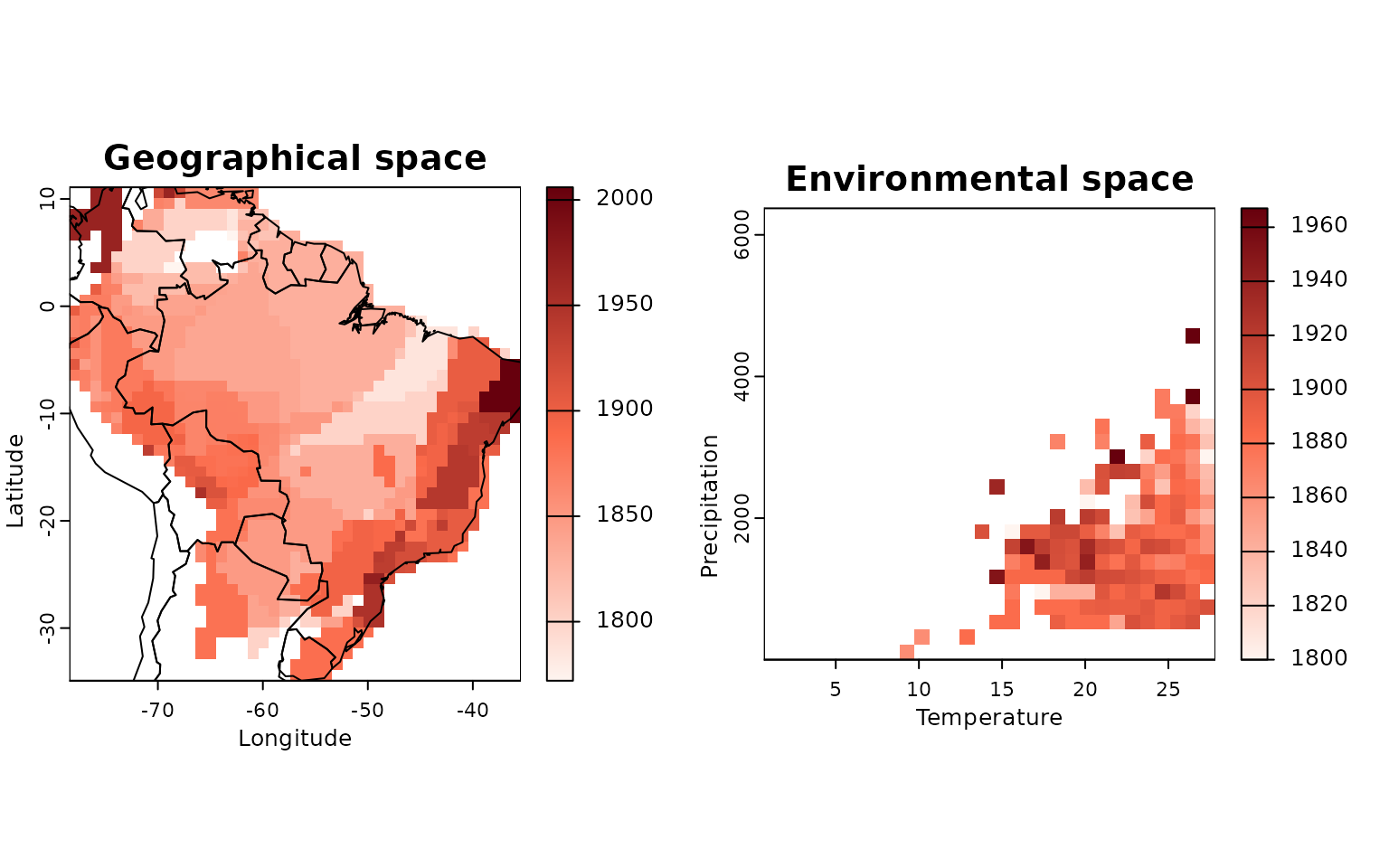
In sum, the lets.envpam() function offers a simple yet
powerful way to explore biodiversity patterns in environmental space. It
enables users to:
- Bin species distributions along ecological gradients.
- Compare spatial and environmental richness.
- Perform niche-based or trait-environment studies.
For advanced analyses, the resulting matrices and rasters can be used in statistical models or overlaid with environmental constraints.
Describing environmental–geographical structure
The object res links geographic and environmental
spaces. We can quantify that structure using
lets.envcells(), which returns per–environmental-cell
descriptors such as frequency (how many geographic cells map to the same
environmental bin), geographic isolation among those cells, distances to
environmental midpoints (negated so larger values imply higher
“centrality”), and distances to environmental borders.
Summarize descriptors per environmental cell
out <- lets.envcells(res)  # perc controls the robust border metric
head(out)
#>   Cell_env Frequency Area Isolation (Min.) Isolation (1st Qu.)
#> 3        1         0   NA               NA                  NA
#> 4        2         0   NA               NA                  NA
#> 5        3         0   NA               NA                  NA
#> 6        4         0   NA               NA                  NA
#> 7        5         0   NA               NA                  NA
#> 8        6         0   NA               NA                  NA
#>   Isolation (Median) Isolation (Mean) Isolation (3rd Qu.) Isolation (Max.)
#> 3                 NA               NA                  NA               NA
#> 4                 NA               NA                  NA               NA
#> 5                 NA               NA                  NA               NA
#> 6                 NA               NA                  NA               NA
#> 7                 NA               NA                  NA               NA
#> 8                 NA               NA                  NA               NA
#>   Weighted Mean Distance to midpoint Mean Distance to midpoint
#> 3                          -3.730908                 -3.457246
#> 4                          -3.646836                 -3.382386
#> 5                          -3.564523                 -3.309862
#> 6                          -3.484092                 -3.239832
#> 7                          -3.405677                 -3.172460
#> 8                          -3.329421                 -3.107918
#>   Minimum Zero Distance Minimum 20% Zero Distance Distance to MCP border
#> 3                     0                 0.9362266                      0
#> 4                     0                 0.8700119                      0
#> 5                     0                 0.8136812                      0
#> 6                     0                 0.7676179                      0
#> 7                     0                 0.7323872                      0
#> 8                     0                 0.7068043                      0
#>   Frequency Weighted Distance
#> 3                    3.800462
#> 4                    3.718461
#> 5                    3.638213
#> 6                    3.559825
#> 7                    3.483411
#> 8                    3.409092
Plot the descriptors
We can plot every descriptor over the environmental raster grid. Optionally, set ras = TRUE to also retrieve the layers as a named list of SpatRaster objects for further use.
lets.plot.envcells(res, out)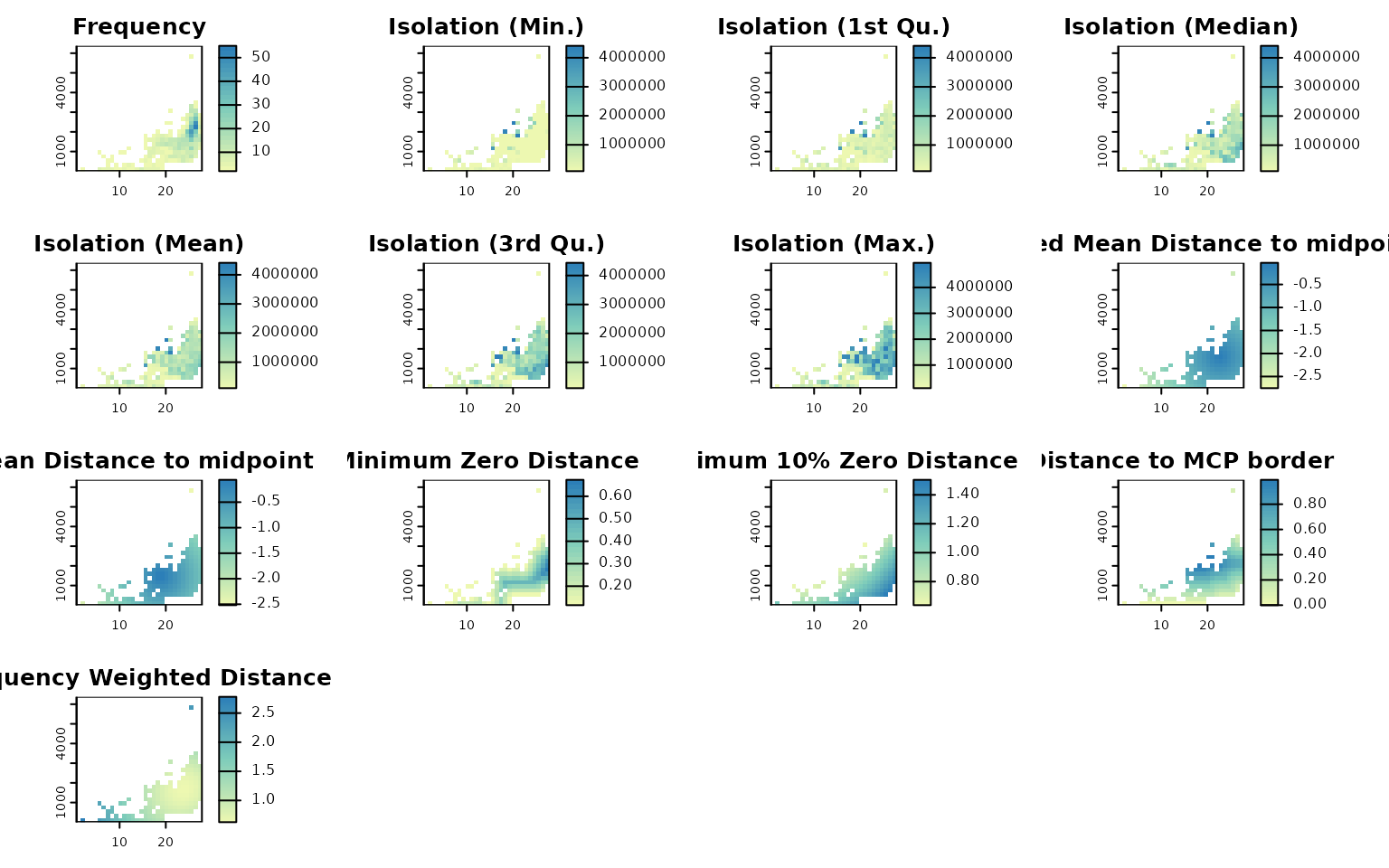
Optionally retrieve rasters for further analysis:
ras_list <- lets.plot.envcells(res, out, ras = TRUE, plot_ras = FALSE)Diagnosing centrality vs. richness (optional)
As a simple diagnostic, we may examine whether environmental centrality (inverse distance to the weighted midpoint) co-varies with environmental richness.
centrality <- out[["Weighted Mean Distance to midpoint"]]   # larger = more central
rich_env   <- rowSums(res$Presence_and_Absence_Matrix_env[, -(1:3), drop = FALSE])

# Mantain cells without zero
keep <- res$Presence_and_Absence_Matrix_env[, 1]
centrality <- centrality[keep]


# Plot relationship
plot(centrality, rich_env,
     xlab = "Centrality (inverse distance to weighted midpoint)",
     ylab = "Species richness",
     pch  = 19)
abline(lm(rich_env ~ centrality), lwd = 2)
These descriptors often reveal whether species accumulate in central portions of environmental space or cluster near edges (where zero-richness neighbors are close), thereby sharpening inference about ecological filtering and range limits.