Mapping species richness in attribute space
Bruno Vilela
2025-07-07
Source:vignettes/Mapping-species-richness-in-attribute-space.Rmd
Mapping-species-richness-in-attribute-space.RmdOverview
Species richness and community structure can also be represented in
attribute space, where axes correspond to any quantitative information
that can be attributed to a species. The letsR package
provides tools to construct and analyze presence–absence matrices (PAMs)
in attribute space, allowing researchers to examine biodiversity
patterns beyond geography and environment.
This vignette demonstrates how to:
- Build a PAM in attribute space using
lets.attrpam(); - Visualize species richness with
lets.plot.attrpam(); - Compute descriptors per attribute cell using
lets.attrcells(); - Aggregate descriptors to the species level with
lets.summarizer.cells(); and - Cross-map attribute metrics to geographic space for integrative analysis.
Simulating trait data and building the attribute space PAM
We begin by generating a dataset of 2,000 species with two correlated traits:
set.seed(123)
n <- 2000
Species  <- paste0("sp", 1:n)
trait_a  <- rnorm(n)
trait_b  <- trait_a * 0.2 + rnorm(n)
df       <- data.frame(Species, trait_a, trait_b)

# Build the attribute-space PAM
attr_obj <- lets.attrpam(df, n_bins = 30)
Visualizing richness in attribute space
The lets.plot.attrpam() function plots the richness
surface across the bivariate trait space.
lets.plot.attrpam(attr_obj)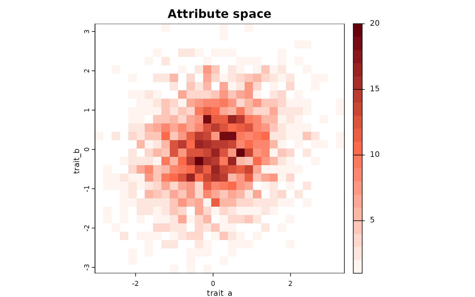
Each cell represents a unique combination of traits (binned values of
trait_a and trait_b), and the color intensity
indicates the number of species falling within that bin.
Computing attribute-space descriptors
The function lets.attrcells() quantifies structural
properties of each cell in the trait space, including measures of
centrality, isolation, and border proximity.
attr_desc <- lets.attrcells(attr_obj, perc = 0.2)
head(attr_desc)
#>   Cell_attr Weighted Mean Distance to midpoint Mean Distance to midpoint
#> 3         1                          -2.326864                 -2.353019
#> 4         2                          -2.249095                 -2.275839
#> 5         3                          -2.174679                 -2.202012
#> 6         4                          -2.103971                 -2.131885
#> 7         5                          -2.037358                 -2.065836
#> 8         6                          -1.975254                 -2.004267
#>   Minimum Zero Distance Minimum 20% Zero Distance Distance to MCP border
#> 3                     0                 0.7875427                      0
#> 4                     0                 0.7238193                      0
#> 5                     0                 0.6742795                      0
#> 6                     0                 0.6362405                      0
#> 7                     0                 0.6116810                      0
#> 8                     0                 0.5974101                      0
#>   Frequency Weighted Distance
#> 3                    2.401182
#> 4                    2.325796
#> 5                    2.253747
#> 6                    2.185353
#> 7                    2.120959
#> 8                    2.060930
We can visualize these metrics using
lets.plot.attrcells():
lets.plot.attrcells(attr_obj, attr_desc)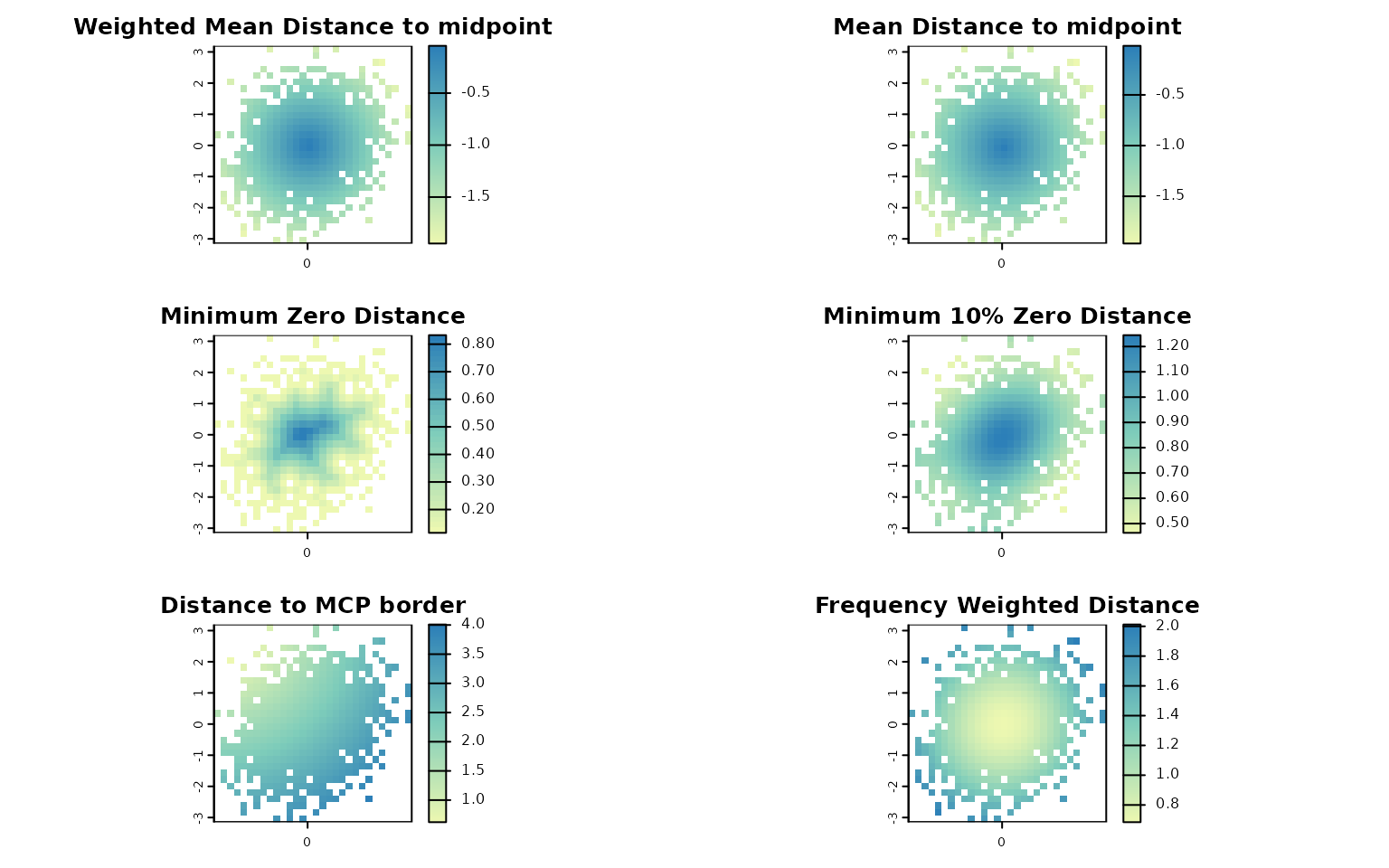
Each panel represents a different descriptor (e.g., distance to midpoint, distance to border, weighted isolation) mapped across the trait space.
Summarizing descriptors by species
To derive species-level summaries, we can aggregate descriptor values
across all cells occupied by each species using the
lets.summarizer.cells() function.
attr_desc_by_sp <- lets.summaryze.cells(attr_obj, attr_desc, func = mean)
head(attr_desc_by_sp)
#>   Species Weighted Mean Distance to midpoint Mean Distance to midpoint
#> 1     sp1                        -0.50820192                -0.4896199
#> 2     sp2                        -0.12253919                -0.1470435
#> 3     sp3                        -0.84093748                -0.8298832
#> 4     sp4                        -0.65172785                -0.6818160
#> 5     sp5                        -0.07626174                -0.1050365
#> 6     sp6                        -0.95462516                -0.9441664
#>   Minimum Zero Distance Minimum 20% Zero Distance Distance to MCP border
#> 1             0.4618802                 1.1195434              1.2701706
#> 2             0.8164966                 1.2218190              1.5011107
#> 3             0.3265986                 0.8310473              0.7745967
#> 4             0.2309401                 0.9311691              1.0392305
#> 5             0.8082904                 1.2360965              1.6041613
#> 6             0.2309401                 0.7661288              0.6733003
#>   Frequency Weighted Distance
#> 1                   0.8225743
#> 2                   0.6921972
#> 3                   1.0446166
#> 4                   0.9069837
#> 5                   0.6857976
#> 6                   1.1319803
This produces a data frame in which each row corresponds to a species, and each column corresponds to the mean descriptor value across the cells where that species occurs. `
Linking attribute space to geographic space
When a geographic PAM generated by lets.presab() is
supplied through the y argument, lets.attrcells() links the
species occurring in each attribute cell to the geographic cells
occupied by those species. This enables the computation of additional
descriptors in geographic space.
data("PAM")

n <- length(PAM$Species_name)
Species <- PAM$Species_name
trait_a <- rnorm(n)
trait_b <- trait_a * 0.2 + rnorm(n)
df <- data.frame(Species, trait_a, trait_b)

x <- lets.attrpam(df, n_bins = 4)

cell_desc_geo <- lets.attrcells(x, y = PAM)
head(cell_desc_geo)
#>   Cell_attr Frequency         Area Isolation (Min.) Isolation (1st Qu.)
#> 3         1       625 7.610774e+12        101354.56            995744.9
#> 4         2         0 0.000000e+00             0.00                 0.0
#> 5         3       104 1.277753e+12        101354.56            435455.5
#> 6         4        15 1.822784e+11        110577.35            156797.2
#> 7         5        72 8.858890e+11         96965.99            322461.4
#> 8         6       497 6.048791e+12         91839.61            857643.9
#>   Isolation (Median) Isolation (Mean) Isolation (3rd Qu.) Isolation (Max.)
#> 3          1642232.9        1747128.1           2384391.6          4749476
#> 4                0.0              0.0                 0.0                0
#> 5           672554.2         722752.7            942685.7          2959492
#> 6           331739.8         644769.6            663456.3          2894931
#> 7           491756.2         513232.8            686374.2          1284485
#> 8          1352699.2        1517451.6           2012096.3          4548857
#>   Weighted Mean Distance to midpoint Mean Distance to midpoint
#> 3                         -1.5126554                -1.5627376
#> 4                         -1.0102709                -1.0708381
#> 5                         -1.1194498                -1.1624284
#> 6                         -1.7279145                -1.7480804
#> 7                         -1.1689967                -1.1913948
#> 8                         -0.3147603                -0.3520894
#>   Minimum Zero Distance Minimum 10% Zero Distance Distance to MCP border
#> 3             0.8660254                 0.8660254              0.0000000
#> 4             0.0000000                 0.0000000              0.0000000
#> 5             0.8660254                 0.8660254              0.0000000
#> 6             1.7320508                 1.7320508              0.0000000
#> 7             1.2247449                 1.2247449              0.8660254
#> 8             0.8660254                 0.8660254              0.8660254
#>   Frequency Weighted Distance
#> 3                    1.988764
#> 4                    1.385760
#> 5                    1.506749
#> 6                    1.928870
#> 7                    1.489442
#> 8                    1.181192
When y is provided, the output includes additional
variables:
-
Frequency: number of geographic cells associated with each attribute cell; -
Area: summed area of those geographic cells; and - geographic isolation summaries:
Isolation (Min.)Isolation (1st Qu.)Isolation (Median)Isolation (Mean)Isolation (3rd Qu.)Isolation (Max.)
These variables allow direct integration of position in attribute space with occupancy and isolation patterns in geographic space.
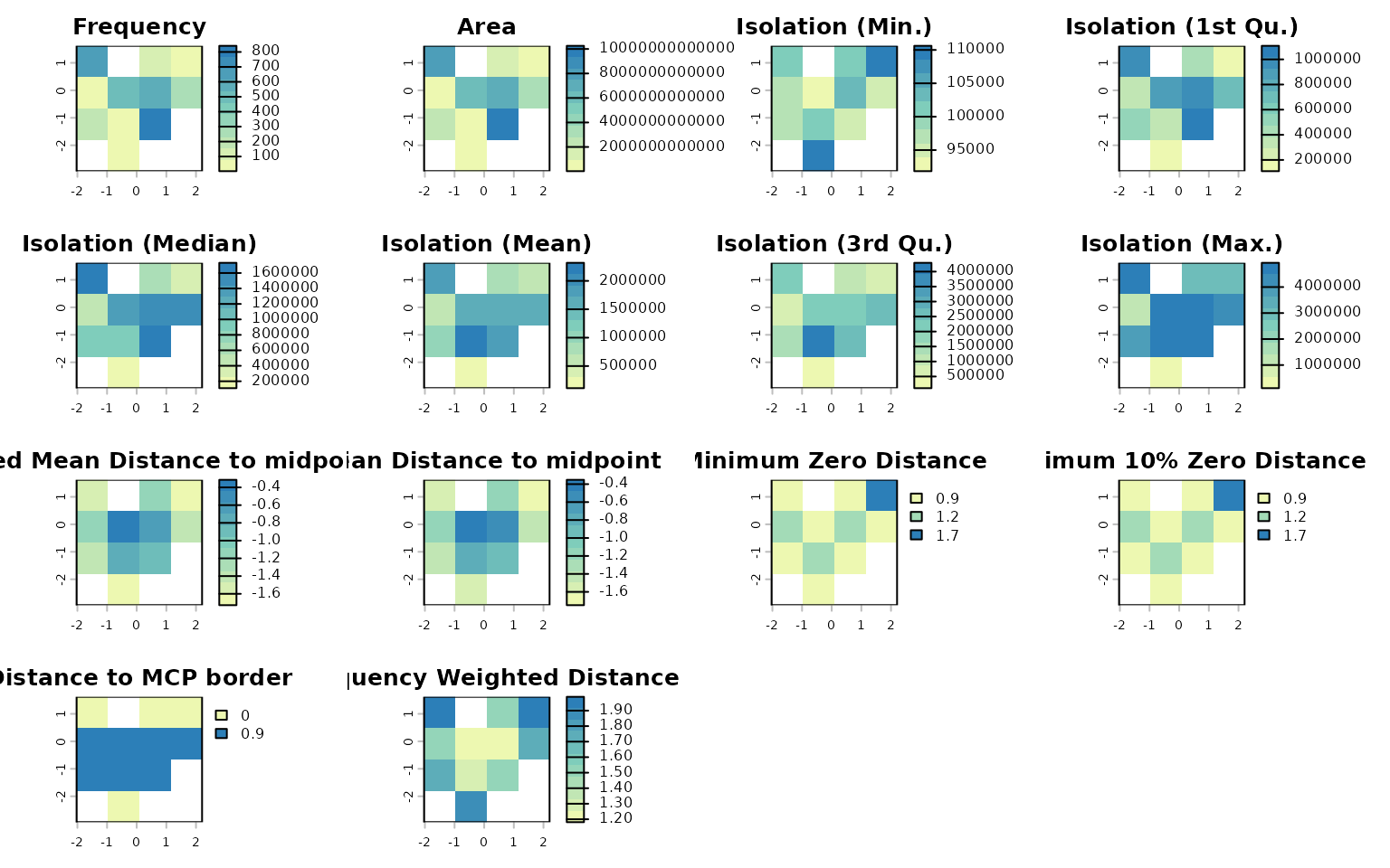
The resulting descriptors can also be plotted:
lets.plot.attrcells(x, cell_desc_geo)